Information & Analysis Documentation

Exploratory Association Figures

Figure 1:

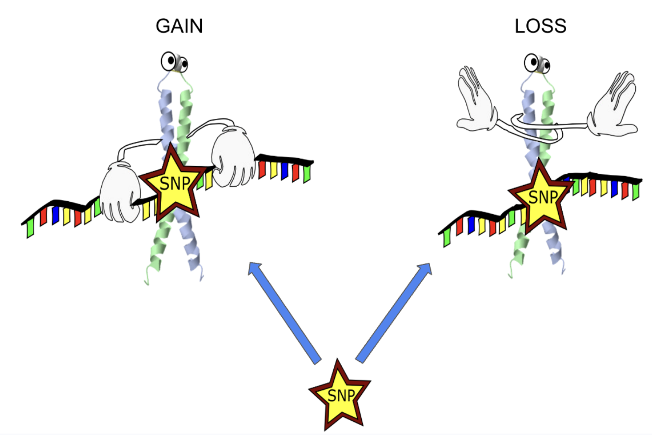
Figure 1. A depiction of the effect that a SNP can have on Transcription factor binding. A SNP (bottom) is depicted as resulting in gain of transcription factor binding (left) and loss of binding (right).

The SNPeBoT family of predictors was initially designed to tackle the prediction of allele specific binding (ASB) events. These events occur when a single mutation (SNP) along DNA will result in a change of Transcription Factor (TF) binding. When a SNP occurs along a DNA sequence it may either change the binding pattern of a TF in. Which NPeBoT family of predictors was initially designed to tackle the prediction of allele specific binding (ASB) events. These events occur when a single mutation (SNP) along DNA will result in a change of Transcription Factor (TF) binding. When a SNP occurs along a DNA sequence it may either change the binding pattern of a TF in which case it must be determined to lead to either a gain or loss in binding or it could have no measurable effect on the TFs binding.

When the SNP changes the binding behavior of a TF it can have downstream effects as well. The genes that the TF regulates from its perturbed binding state at that given genomic coordinate can consequently also see changes in expression. When the alteration of the expression of these genes is signifiant enough to have phenotypic consequences it can be said that the SNP and ASB are of medical significance. It therefore becomes of great importance to be able to identify these SNPs. This is what we have tried to achieve.

Figure 2:

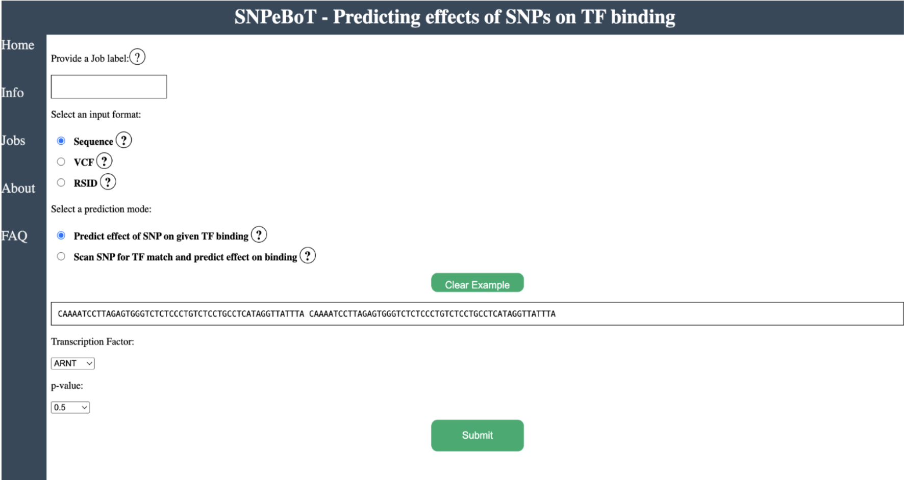
Figure 2. A screenshot of the Home Screen of the SNPeBoT website.

In a previous work we developed and published SNPeBoT. SNPeBoT can be accessed through the url (https://snpebot.upf.edu/). Like SNPeBoT2 it will take as TF information as well as reference and alternate binding sequences and predict if the SNP on the alternate sequence will perturb the binding of the selected TF or scan for a TF to use on its own.

Figure 3:

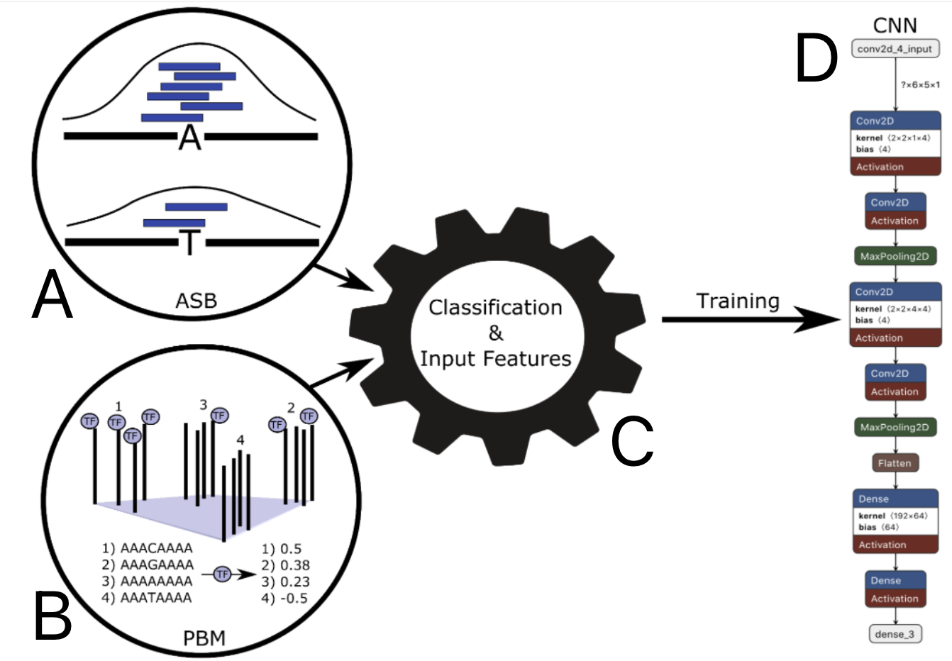
Figure 3. An outline of the structure of the SNPeBoT predictor. A) ASB events are taken from experimental data and combined with B) PBM Escore data of a subset of possible TFs. C) the data is combined in order to create input features for D) a CNN that will predict if the SNP from the ASB data will result in gain, loss or no change to the binding of the selected TF.

The SNPeBoT design was limited by its reliance on PBM data to generate the data needed to train and run the predictive model. Due to this limitation any TF that had not undergone PBM experiments and consequently had no E-score values associated with it could not be handled by SNPeBoT. While the SNPeBoT predictor performed quite well on the TFs that it could predict on this limitation prevented broader applicability.

Figure 4:

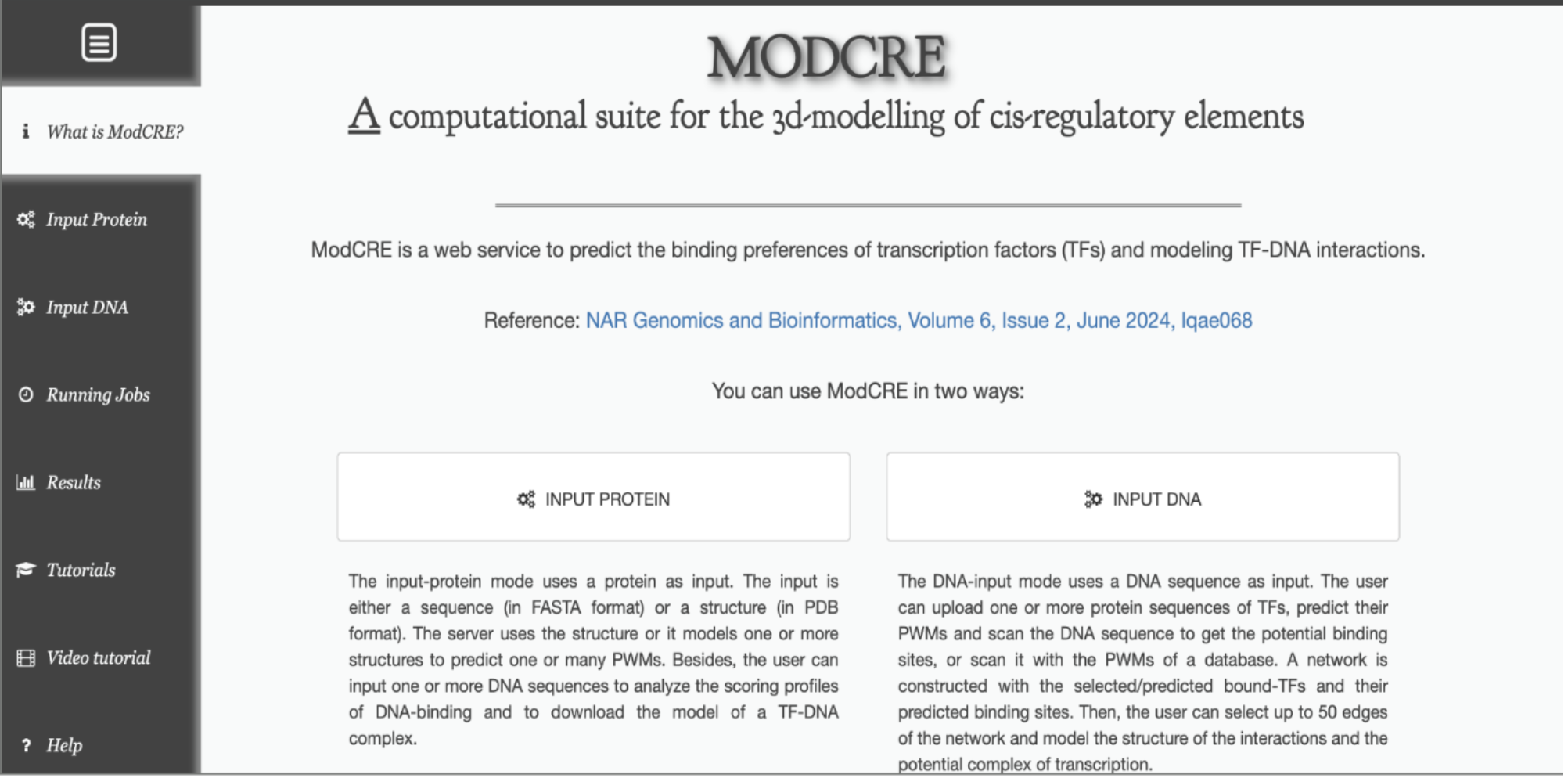
Figure 4. A screenshot of the ModCRE Home Screen.

However ModCRE (http://aleph.upf.edu/modcre/) presented a solution to the problem faced by SNPeBoT. It is capable taking an amino acid sequence of a target TF as input and generating a 3D model of that TF binding DNA. This 3D model is then used by ModCRE do generate statistical potential scoring profiles for the binding of the TF along any input DNA sequence.

In order to apply the ModCRE approach to the issue of ASB predictions it had to be adapted. ModCRElib (https://github.com/structuralbioinformatics/ModCRElib) was developed, a standalone package adapting ModCRE methods to high throughput jobs as well as extending its functionality.

Figure 5:

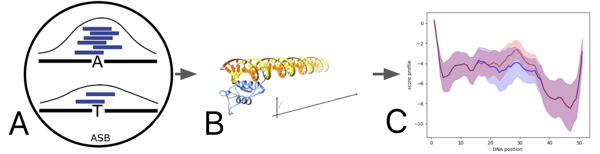
Figure 5. A figure depicting how ModCRElib can be applied to ASB data. A) ASB data is used for preparation of wildtype and mutant sequences. B) Each sequence is put through the ModCRElib pipeline to generate statistical potential profiles. C) Statistical potential score profile comparison between wildtype and mutant sequence for a known ASB event.

Like with SNPeBoT, the training and testing data for SNPeBoT2 is derived from experimental ASB data. However, due to the shedding of PBM data requirements the data upon which to train SNPeBoT2 is increased. The wildtype and mutant sequences are then put through ModCRElib to generate statistical potential scoring profiles. Like with SNPeBoT multiple snapshots of the region including the SNP are taking for profiling. The profiles of the wildtype and mutant sequences can then be compared.

Figure 6:

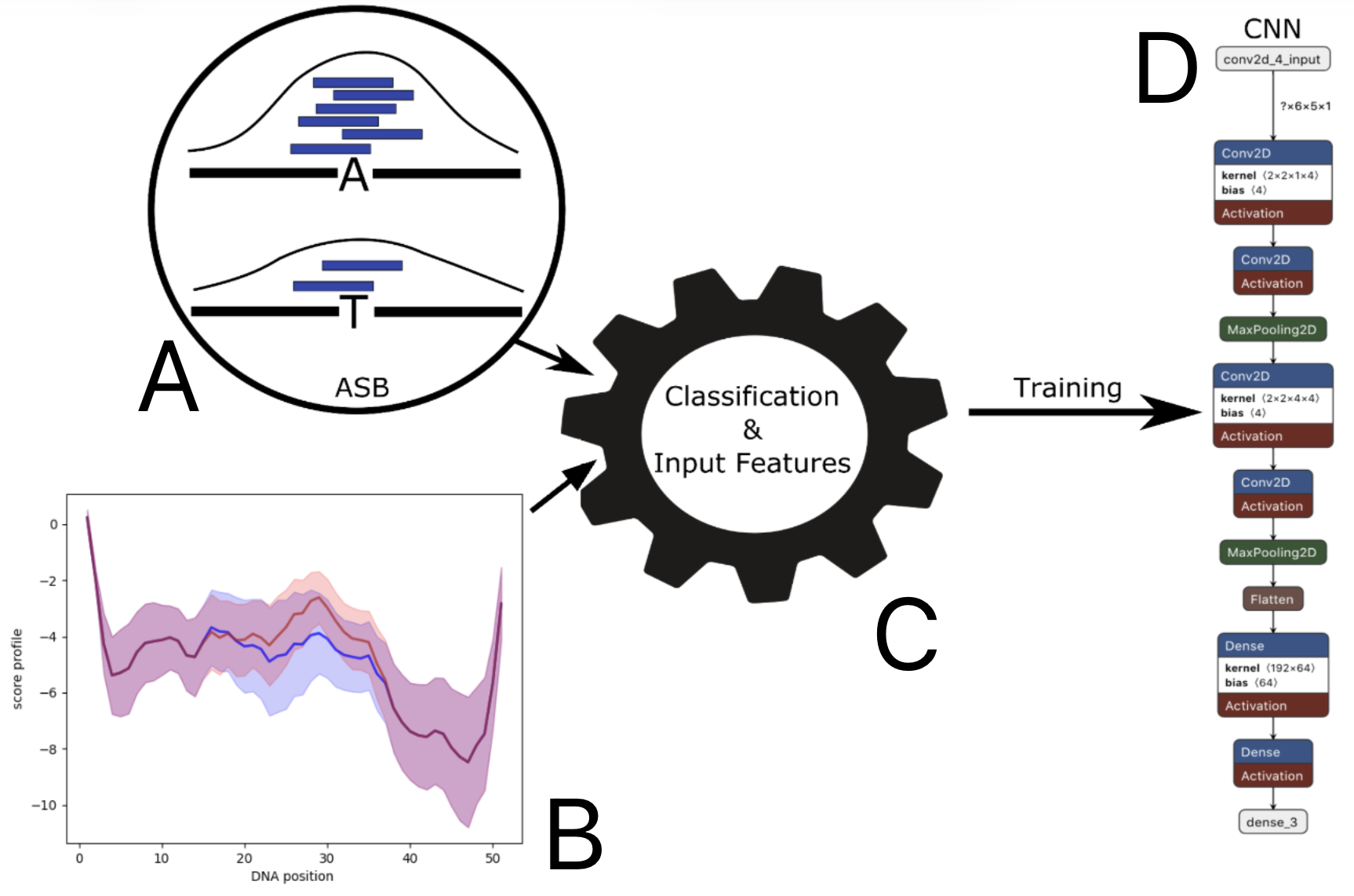
Figure 6. A figure of the architecture of the SNPeBoT2 ASB predictor. A) ASB data is used to generate B) statistical potential score profiles for wildtype and mutant sequences. C)The statistical potential scoring profiles are merged and processed for downstream training and prediction. D) The architecture of one of the two identical CNNs predicting the class of the input.

The architecture of the SNPeBoT2 ASB predictor is very similar to that of SNPeBoT shown in figure 3. However, there is one major difference and that is the replacement of PBM data with the statistical potential scores generated with ModCRElib. Because ModCRElib needs only an amino acid sequence of a TF as input in order to generate its scoring data any TF can be applied.

With respect to SNPeBoT its successor, SNPeBoT2, is a completely different model. Aside for the change in how ASBs are converted into input features there is a difference in the training data, the model architecture and the model was also able to be tested on different data sets.

Figure 7:

Figure 7. Performance of the SNPeBoT2 ASB predictor on various different benchmarks. a) a scatterplot showing macro averaged 3 class prediction accuracy on the x axis and the ASB recall rate on the y axis. Plotted are the performances of the Benchmarking tools as shown in the SNPeBoT paper and SNPeBot itself at several different thresholds. To compare, the performance of SNPeBoT2 is plotted as well. C) A normalized confusion matrix of the predictive performance of SNPeBoT2 on the test data from the SNPeBoT paper. This data had PBM E-scores associated with every TF tested. B) a normalized confusion matrix of SNPeBoT2 predictive performance on test data that did not have PBM data associated with any TF included in the dataset.

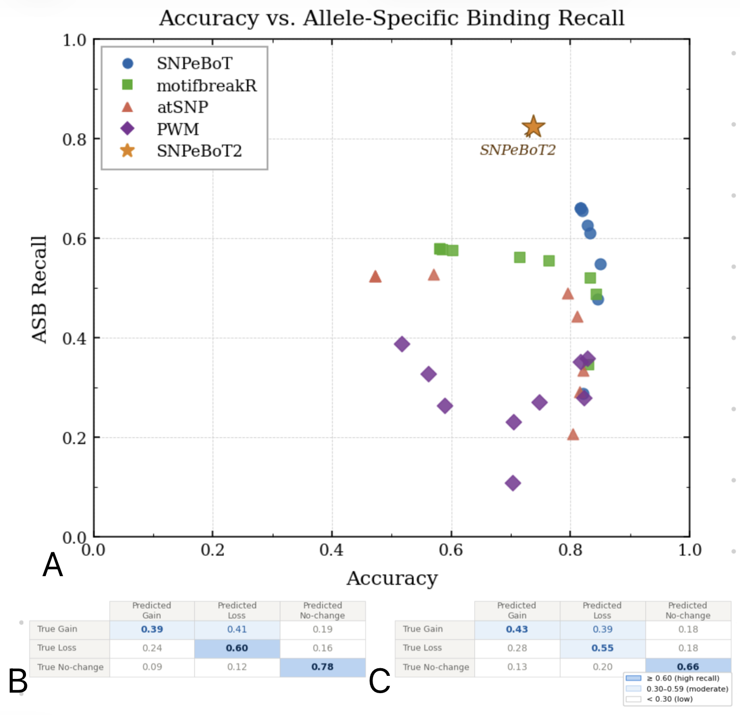
To evaluate directly how well SNPeBoT compare to SNPeBoT and other available ASB predictors we first applied it to the test set of PBM available ASB data from the SNPeBoT paper. As can be seen in Figure 7 the ASB recall rate of SNPeBoT2 was higher than all other models tested. The macro averaged accuracy of SNPeBoT was only marginally lower than the best thresholds for the other models meaning that an increase in ASBs recovered came at only a slight cost to predictive accuracy.

When looking closely at the performance on the PBM ASB data in B of Figure 7 we can see that SNPeBoT2 was able to distinguish quite well between the cases where a SNP resulted in perturbation of TF binding compare to those that cause no change. In contrast it had a harder time distinguishing between gain and loss. This is also reflected when SNPeBoT2 is applied to a seperate test set of ASB data that did not have associated PBM data. While the misclassification of perturbation directionality is present it is much more important that the number of false positive predictions (when viewing the problem as a binary change or no change in binding prediction) remains low. Changes in TF binding on its own can indicate whether a SNP is relevant for downstream regulatory effects. Further examination can then be used to differentiate between the directionality if the reduced accuracy of SNPeBoT2s predictions is not enough.

Figure 8:

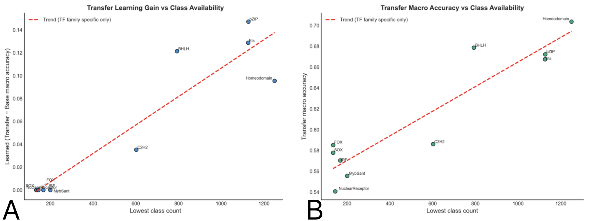
Figure 8. Scatter plots of the performance of transfer learning for SNPeBoT2. A) A scatter plot for select TF famiilies that were used for transfer learning with the data available for training plotted on the x-axis and the learning rate (transfer model performance - original model performance) plotted along the y axis. B) Macro Averaged Accuracy (x-axis) of the transfer models for each of the selected TF families plotted against the data availability (y-axis).

In order to give the SNPeBoT2 model some flexibility we applied transfer learning to fine tune it to family specific models. The ASB data scarcity disallowed the generation of TF family specific models for all TF families. Instead the top 10 TF families were selected for testing the fine tuning. As the results in Figure 8 show, fine tuning was successful, with the fine tuned models outperforming the base model in cases where there was sufficient transfer learning data. However this highlights the pattern observed, where the performance of the transfer model is greatly reliant on the amount of data available.

We have supplied python code for users to apply transfer learning to the SNPeBoT2 model in cases where they believe they have sufficient data to do so. This affords SNPeBoT2 with a flexibility, which means that it can be adapted to whatever task is required by the end user.

Figure 9:

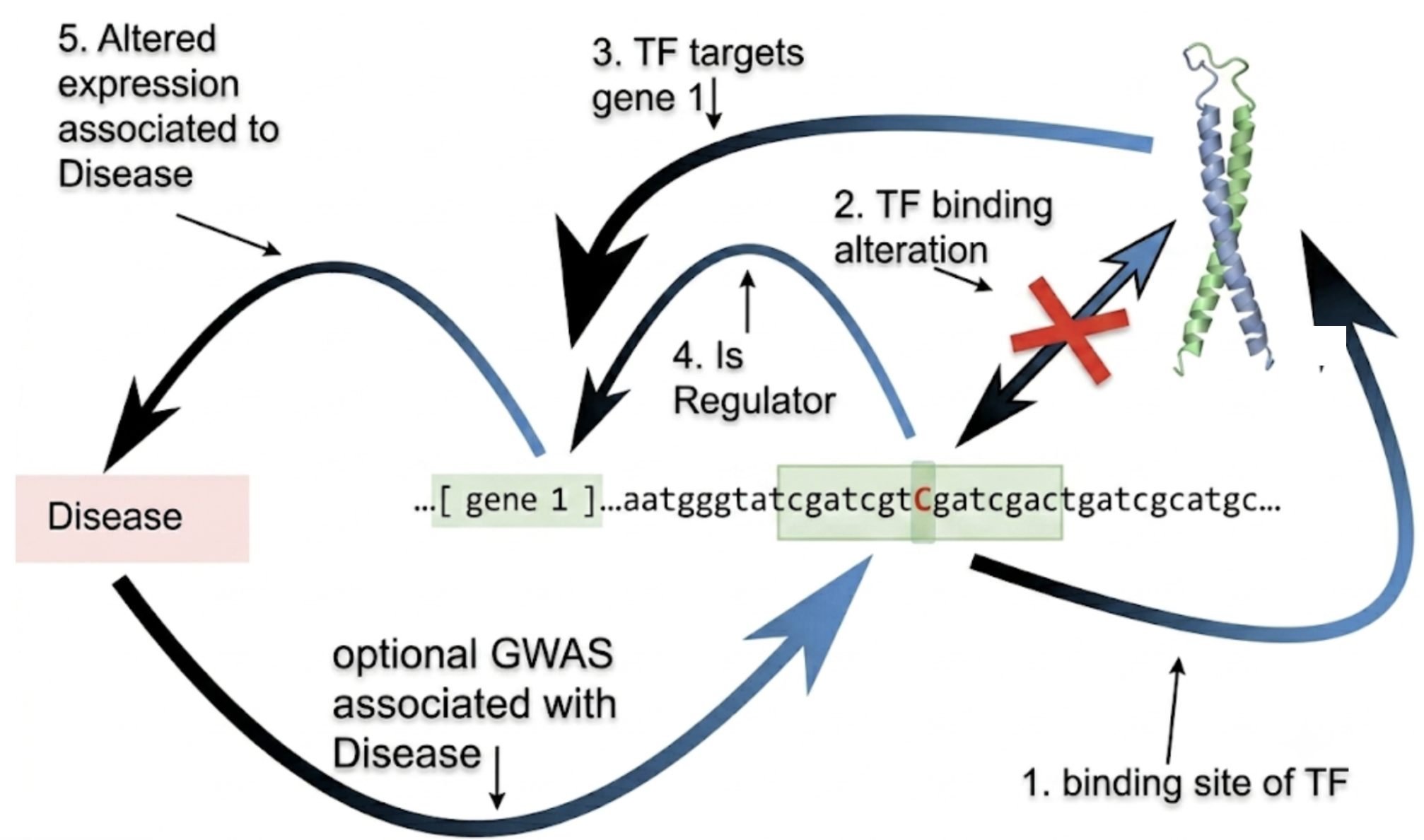
Figure 9. A diagram of the workflow of the Disease-SNP association relevance filter. The various steps are 1) a SNP is a binding site of a target TF which 2) is predicted by SNPeBoT2 to see binding perturbations due to that SNP. 3) TFLink selects which genes in the SNPs proximity are known targets of the TF in question and 4) the ABC model predicts that the site of the SNP is a regulator of those genes. Finally DISGENET 5) provides information on which gene has diseases associated with it when it experiences altered expression.

To further process regulatory SNPs we designed a filtration process to order SNPs according to how likely we determine the SNP to be involved in disease etiology. Every SNP receives scores for their SNPeBoT2 prediction, ABC regulator prediction, gene proximity, and gene-disease association. These are then ranked according to their completeness. While this is not a definitive selection of regulatory SNPs that cause disease it provides a filtration of SNPs down to the ones that should be the most interesting for further investigation. After associations are scored, the user can also decide to run a quick enrichment analysis to see what Biological Processes and Molecular Function terms are enriched in the associations receiving a full completeness score.

Figure 10:

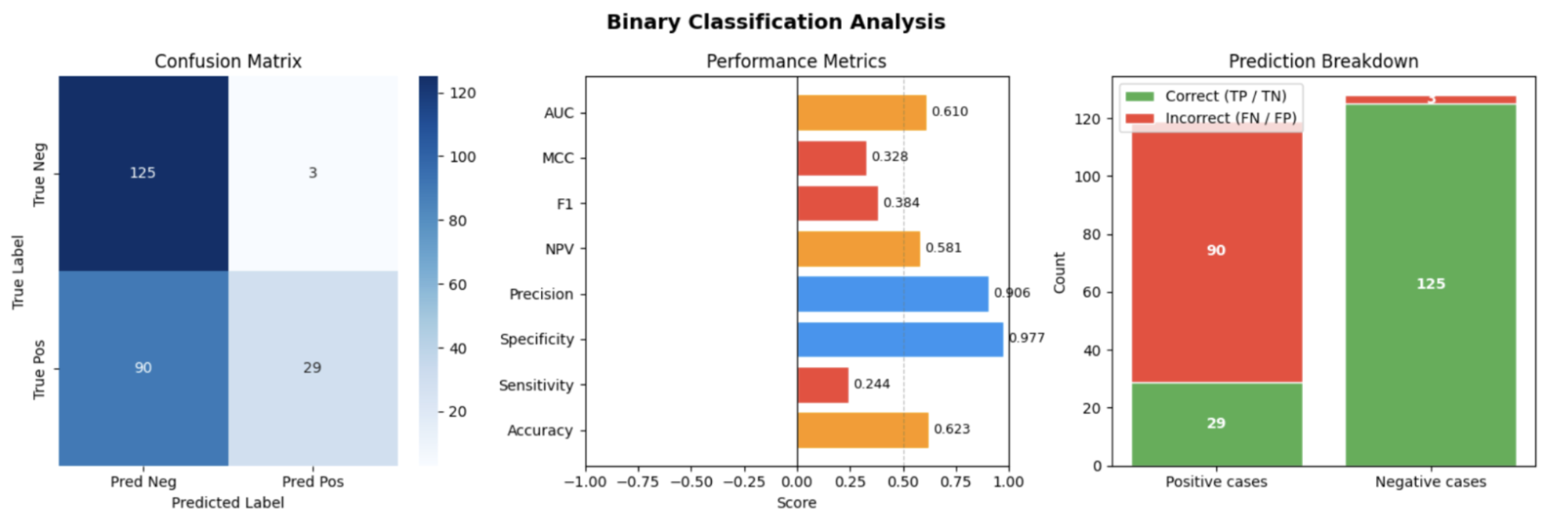
Figure 10. Binary classification analysis of the regulator prediction from the ABC model. A confusion matrix of expected and observed predictions. A barplot of the performance metrics of the tested prediction as well a prediction breakdown showing the recall rate for positive and negative cases of regulators.

To test the ABC models applicability within SNPeBoT2's disease association pipeline we applied it to a known regulators. It predicts enhancers with high precision and specificity which keeps the number of false positives at a minimum.

Figure 11:

Figure 11. A table showing the filtration steps reached of each of the 15 rsids tested. SNP effect is labelled 1 in cases of gain or loss prediction and 0 when no change was predicted. Completed pipeline is labelled 1 when a full completeness score was reached with the association analysis and 0 when not.

A random selection of 15 rsids were selected to demonstrate the full SNPeBoT2 pipeline. Of these, 8 received a positive perturbation prediction and 5 achieved a completeness score of 4.

Association Analysis Output Headers

Describing each column found in the association anlalysis output csv file.

Headers for the csv output files generated by the association analysis are outlined below:

Column Header Field	Data Representation	Functional Analytical Meaning / Context
`TargetGeneSymbol`	String	The official HGNC approved gene short name character symbol mapping identifier closest to the variant locus coordinate points.
`TargetGeneID`	Integer	NCBI Entrez Gene database system global alphanumeric key record parameter locator used for systemic reference cross checks.
`SNPeBoT2_prediction`	Categorical	SNPeBoT2 predicted binding impact classification showing directional influence markers mapped as either `gain` , `loss` , or`no-change` parameters.
`gene_distance_bp`	Integer	The linear genomic distance measurement window counted explicitly in base pairs separating the targeted variant element from transcription start sites.
`regulator_score`	Float	0 for an ABC model derived classification of the SNP residing on a regulator of target gene. Score of 1 indicating it does occur on a regulator.
`regulator`	String	Boolean indicating if the ABC model predicted the SNP to occur on a regulator of the target gene.
`disease_name`	String	The Disease name that DISGENET found to be associated to altered expression of the target gene.
`pmid`	String	The pmid supporting the DISGENET derived disease association with the target gene.
`completeness_score`	Integer	The final integrated structural profile composite confidence index measurement score value evaluating target variant processing pipelines.

Enrichment analysis output

Enrichment analysis for a quick overview of association results.

For each job, the pipeline produced: (i) a per-direction weighted gene table; (ii) a combined enrichment results table spanning all directions and library categories, in both CSV and JSON formats; (iii) a disease provenance summary in JSON format; and (iv) summary bar plots of the top enriched terms per direction–category combination, ranked by −log₁₀(adjusted p-value).

SNPeBoT2 Supporting Documentation and Information